Tutorial 1 - Building a Solar Scenario

Initial Setup

As part of initial project setup, you will need to choose a unique name for your project. You may not see an account selection dropdown; this is a feature available to advanced users. You will also need to select the location of your project; this can be anywhere on earth. This sets the default location of wind and solar installations and what weather data will be fed to the gas turbine model if available on your plan.

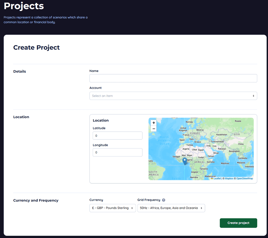
Select a currency and a grid frequency, this influences what generators are available, due to their different running speeds.

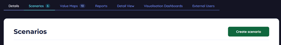
Navigate to the scenario's tab and press “Create Scenario”

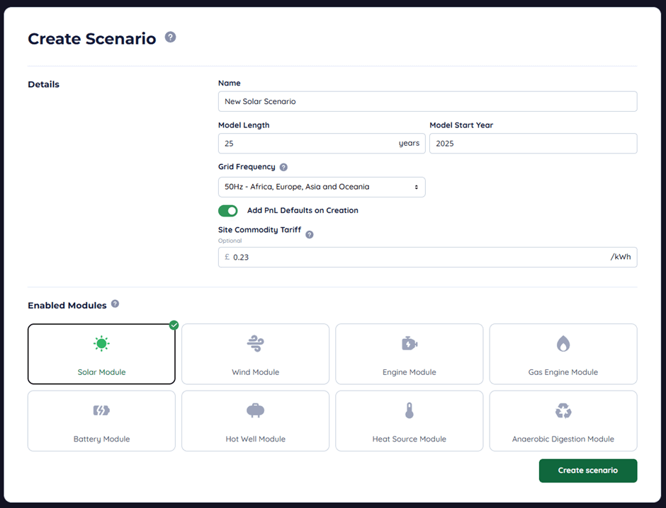
In this example, we are going to be creating a simple solar model. Enable the relevant module and fill out the form. “PnL Defaults” are a selection of commonly used profit and loss entries used in each simulation module, these populate enabled modules when you create the scenario.

These defaults can be added later if you decide to add another module, and they do not already exist.

Value Maps

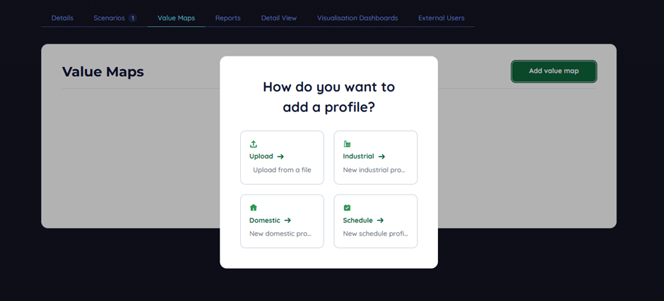
Value maps are a powerful way to collect, store, and input large datasets for use by the model. There are many ways of adding them to the scenario; the most common is importing a csv file in one of the correct formats. We also profile wo profile generators, one industrial profile generator, and another domestic profile generator specialised to the United Kingdom’s TDCV values provided by the energy regulator. We are continuously expanding this facility and welcome feedback on additional generators and methods we could implement.

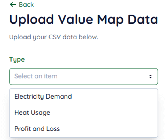
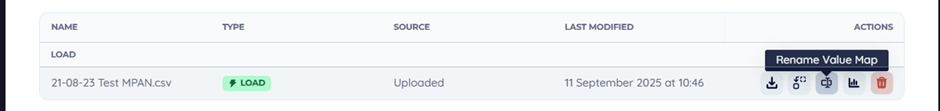
Select the type of value map you wish to create. The name of the profile will be inherited from the name of the file you upload. They can be renamed.

Please ensure the date format and separator character match the file, and that if your metering data is in average demand not metered use that the conversion is applied. Encast works on an Energy basis, not a power basis.

Generating an Industrial Profile

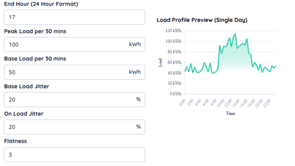
When generating an industrial profile, it will generate the same load every day. This is intended to give a quick variable estimate if you have not created a more complex model of an industrial sites loading and design.

Jitter is an element of randomness in the base and peak load, and flatness gradually reduces the curvature of the load between the start and end hours.

Creating a Demand Entry

To complete the process of defining a load in the scenario, navigate to the scenario through the scenario tab, then click the tab for electrical demand.

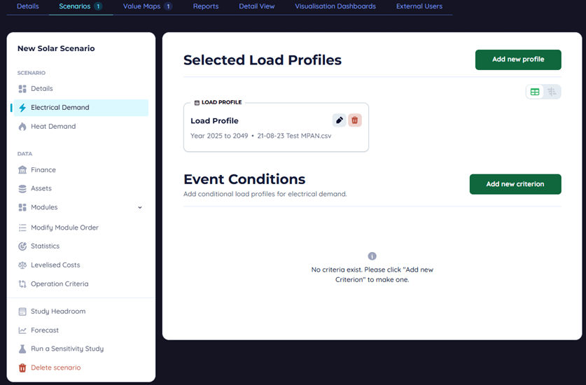
Hit Add new profile to get started on adding a new entry, then give it a name and select the load profile you uploaded earlier. The start and end year select when the profile begins and ends, not that this means they run from the 1s of January to the 31st of December, inclusive of the entire start and end year. You may also set an annual change in demand. This value may be positive, negative, or zero to reflect gradual changes across the site's demand profile.

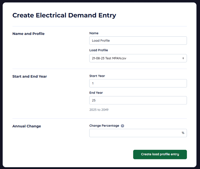
Additionally, multiple profiles can be active at once and will overlap and aggregate together. Value maps can also be set to negative values, while this is not advised, it may be relevant in narrow cases where generation or feed in is occurring in a way that is not modelled by Encast.

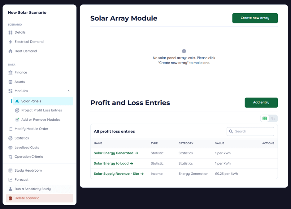
Building an Installation

Now we will need to add an installation to satisfy the demand we just defined. Navigate to solar panels and hit “Create new array”

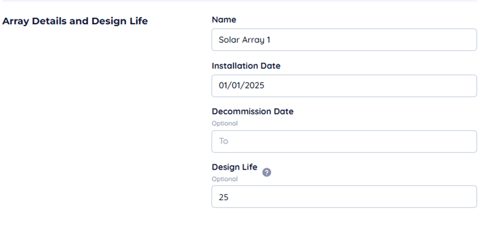
In the form give it a name as usual and state when the array is expected to be installed, in our case it’s installed the first day of the project. Design life is how long the installation is expected to last before being retired, you can also optionally state a specific date.

Select a panel, and the quantity. You can select the project location as a default for the array location or input it yourself. Selecting the optimal panel angle and aspect is recommended if you are using a fixed panel, though for roof-mounted solar you will likely have to adjust this.

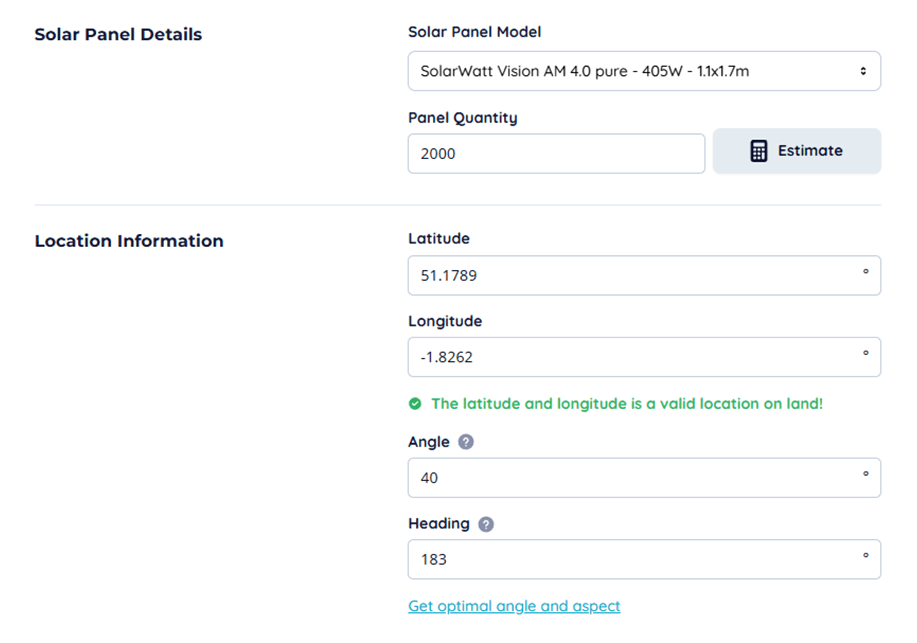
Losses account for the operating dynamics of a solar array. These can vary, and we take a static percentage to account for these. You can also select a variety of tracking functions if you have solar tracking tables, building integrated panels have different responses to ambient temperature, and you can toggle this on or off.

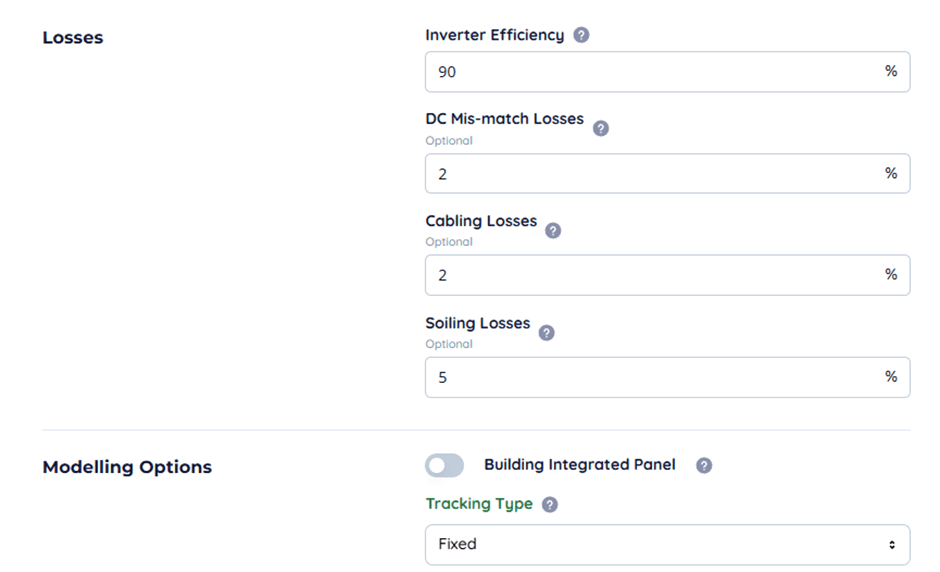
You can ignore the operational times and maintenance sections if available for now.

Profit and Loss Entries

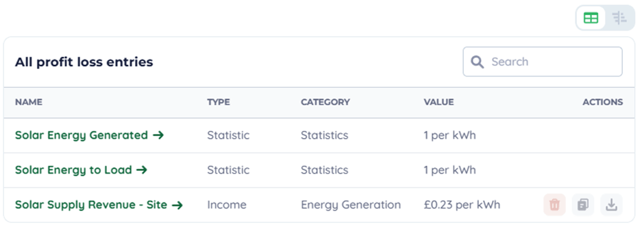
The profit and loss defaults generally comprise the following entries working off the solar array output.

Depending on your plan, you may have the advanced complexity level available. It is advised you do not enable this as the features contained are not relevant to this tutorial. The entry type determines where on the financial report it appears and is accounted for. Carbon entries appear only on the carbon report.

Internal benefits are reductions in operating costs for the site because of the project improvements, these do not affect cash-flow but instead count towards the net present value of the project. In a solar power context, the energy used on site would be an internal benefit, whereas the energy exported and maintenance costs would not.

The value divisor is used to allow the profit and loss entry to count every X of something. Say, for example, a fuel tanker costs a fixed amount every 30,000 Litres you would set the divisor to 30,000.

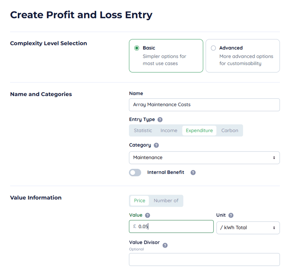
In this example we are using a flat rate of operation, and maintenance costs of £0.05/kWh generated by the array.

Finishing Up & Performance Metrics

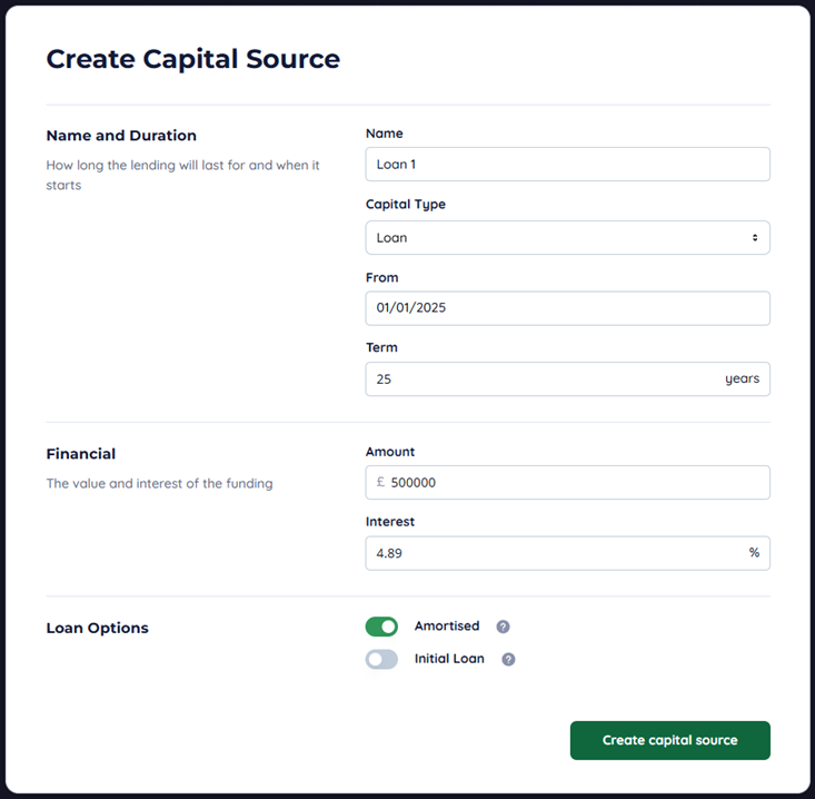
To complete the financial model, setting up some capital sources and assets may be required.

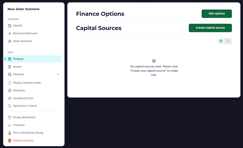
A capital source can be treated as a loan or some other deal structure. Amortisation is a toggle to say whether the principle of the loan is repaid or not, an initial loan does not exist in the cash flow and is treated as having existed at the project start.

The financial settings primarily affect taxation and the discount rate of the financial analysis. For our model “tax rate” is the equivalent in structure to UK corporation tax. You can also see the site commodity tariff value if you didn’t at scenario creation.

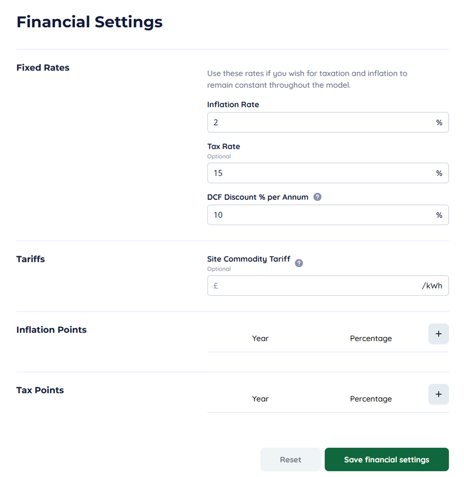
Use the points to set up variable tax rates and inflation rates across the model if you do not want to use a flat value throughout.

The Reports Page

This page is used to present the high-level output of the model.

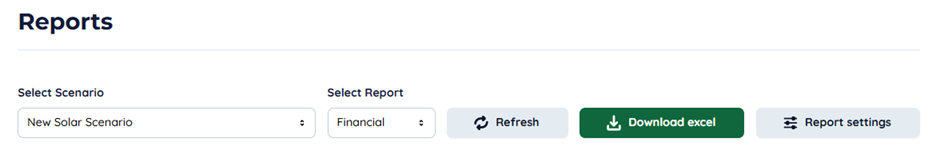
Select the scenario you want to see and select one of the reports, then hit refresh. This will run the scenario in real time and should take less than 5 seconds.

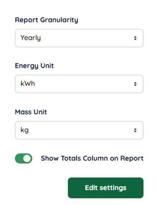
You can choose to change energy and mass units and toggle the total column in the options. Report granularity allows you to see month-by-month breakdowns of a single year.

Graphing

As a demonstration of the graphing system, we are going to create a daily time series output of the solar output. Navigate to the dashboard page and select create dashboard and fill in the form.

Click “Go to dashboard”, then “Create chart”.

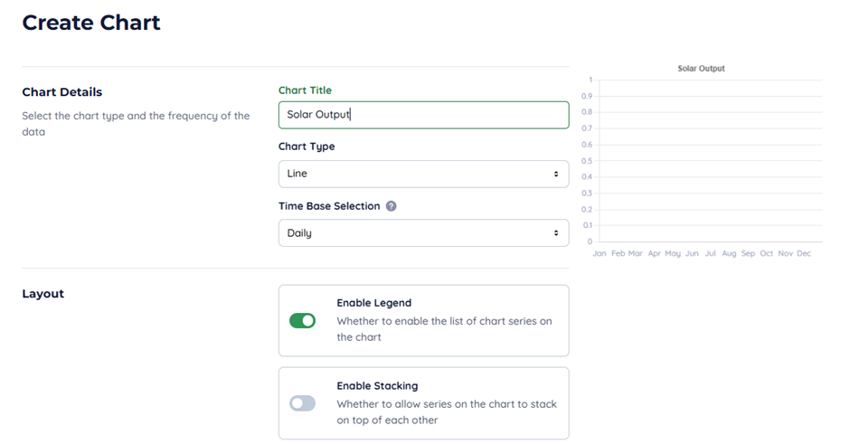
Set the chart type to “Line” and the time base selection to “Daily”. Scroll down and hit “Add series”.

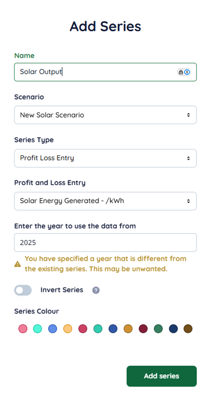
Select the profit loss entry for solar energy generated and use the data from the first year, remember to select a colour.

<

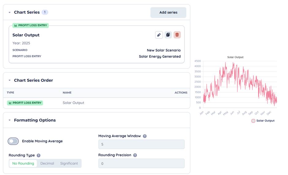
You will notice that the intraday variance of solar output causes the graph to be challenging to understand. To resolve this, you can add a 5-day moving average.

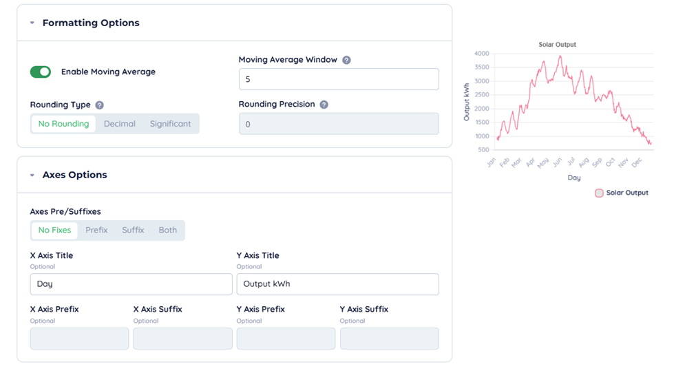
You can also add axes titles if you wish. Then press the chart creation button.

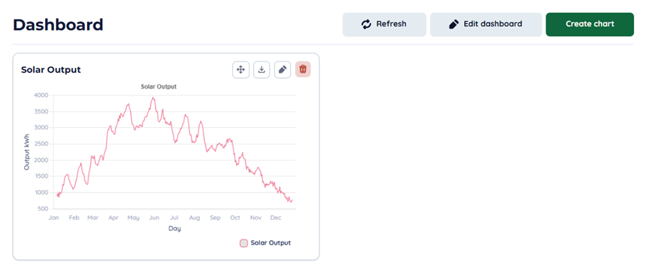
Now you should see your new graph in the dashboard. Once submitted, hit refresh to render the chart if it does not already, you can edit and download the chart using the action buttons in the top right of the tile.

Adding New Modules

To add new modules to an existing project, click “Add or Remove Modules” under “Modules”.

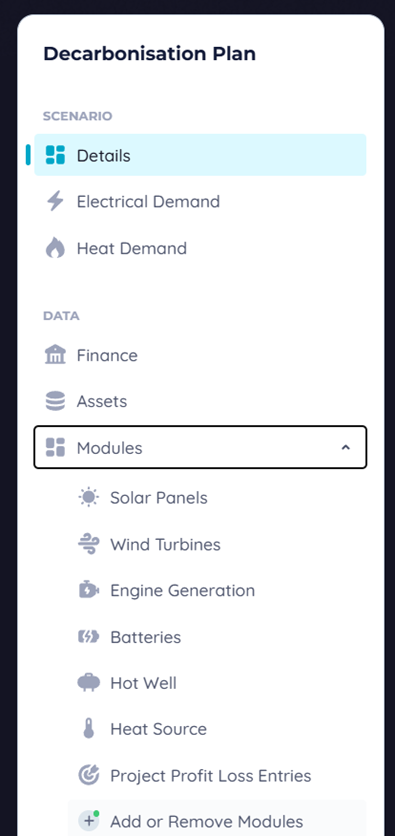
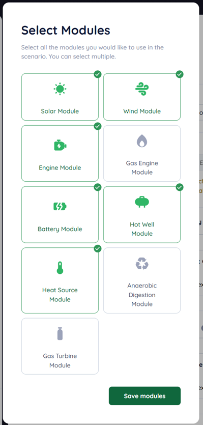
Then select which ones you want and click save modules. If you deselect a module and save, you won’t lose any installations or profit and loss entries you have selected in that module, they simply will be disabled in the model.

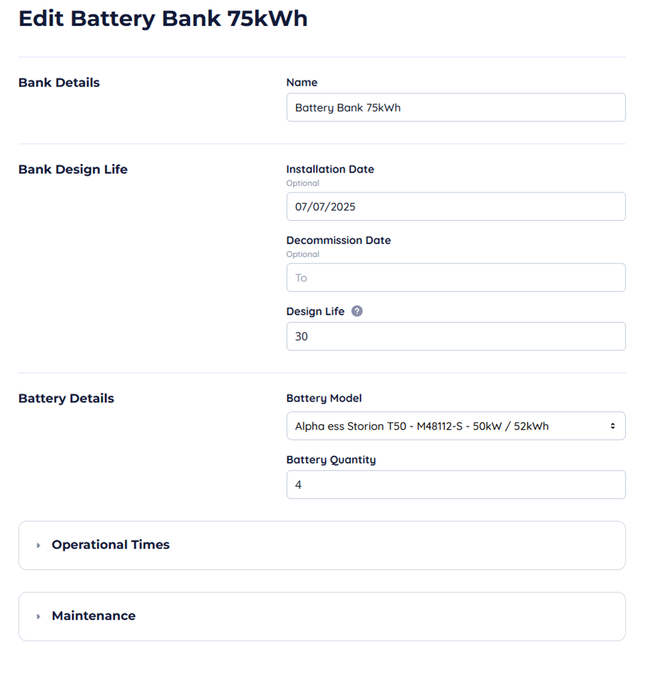
Batteries

Batteries are a fantastic way of managing renewable and in advanced scenarios performing tasks like peak shaving. Though they can do a lot of things, setup is straightforward. Select a battery model and the number you want after entering the design life. Note that battery life is highly important and is a parameter within the battery itself, usually this is 10–15 years depending on usage. Please check the datasheets for each model of battery you want to use if you are unsure how this could affect your project.

Generators

Generators of any type are some of the more complex modules in Encast and have a multitude of parameters that need to be determined before it will function. The details and design life should be familiar to you, so we will focus on engine details and running properties.

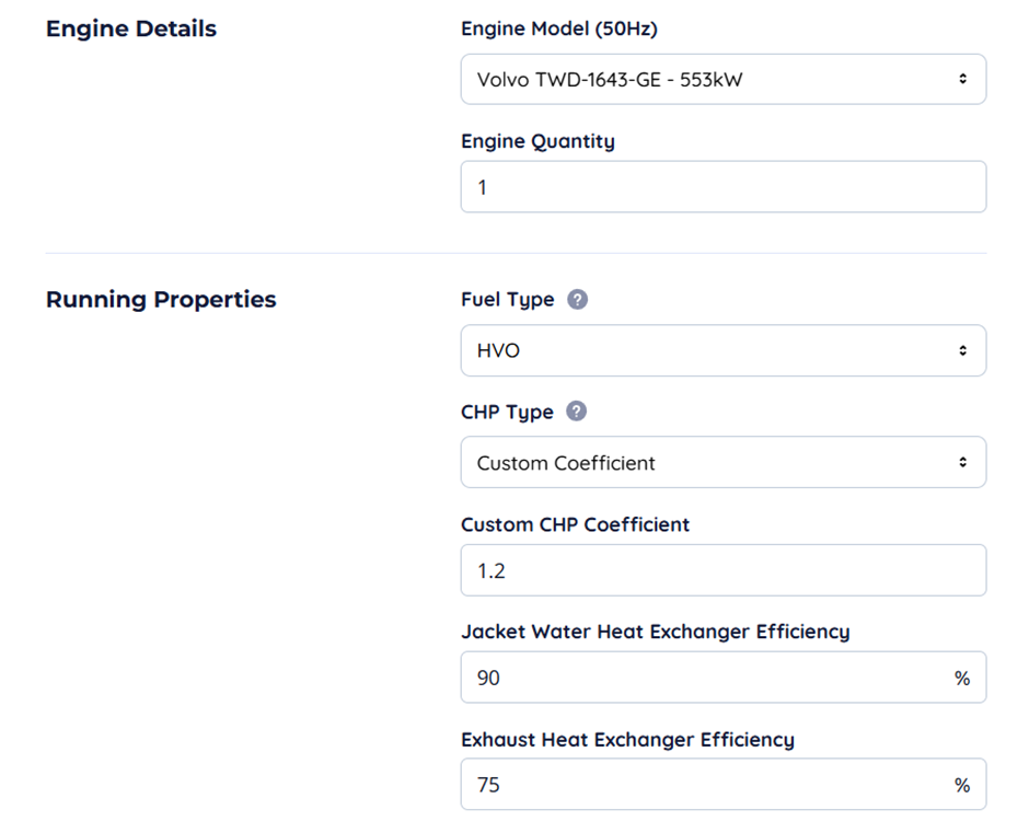
Fuel type is one of the most important parameters, in this instance HVO has been selected. The fuel type affects both the specific gravity and energy density of fuels effecting fuel consumption; it also affects the efficiency of the engine. A custom CHP coefficient has been selected this will override the coefficients selected by the engine to reflect custom or nonstandard heat recovery methods. You can select the heat exchanger efficiencies, alternatively you can completely remove CHP if it’s not planned to be fitted to the engine.

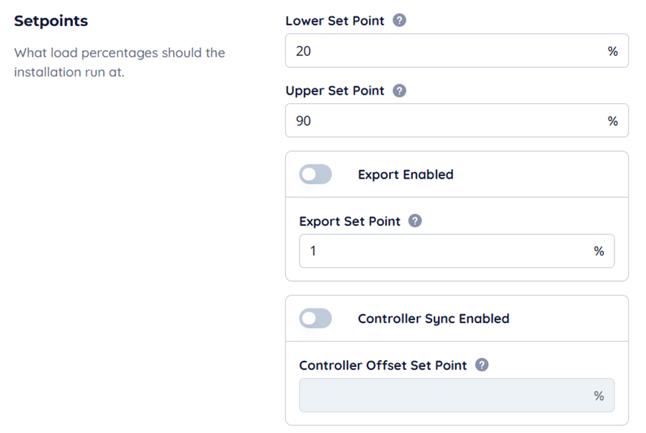
The lower and upper setpoints allow you to control the point below which the engine will shut down and the upper setpoint which is the maximum throttle. These are all expressed in the percentage of the engine load. These setpoints are critically important when operating on sustainable fuels as the differing characteristics of the fuel from diesel will quickly destroy the engine if placed under too much load. At lower throttle levels gumming and other undesirable effects can occur, even without fouling the engines are much less efficient outside the setpoints.

The export-enabled flag allows the engine to run regardless of the incoming load and on startup will run as long as possible up to the export set point. Controller Sync offset is used to model the amount of power used by the generator to energise its own alternator windings and contributes to the parasitic load which is again defined by the engine.

Gas engines operate in the same way, however, have a slightly less complex CHP heat availability calculation.