Tutorial 2—Module Overviews and Problem-Solving

This tutorial is intended to demonstrate more of the features available in the standard licence plan and provides a basic overview of how to use them to solve problems in the project.

Grid Sizing

We have two different parameters that represent the capacity of the connection for a scenario to the wider electricity grid, these are both measured in kilowatts. “Export Capacity” is the amount of energy that can be exported from the site. Likewise, “Incomer Sizing” defines what can come onto the site. If you don’t care about the size of the connection, you can leave both blank.

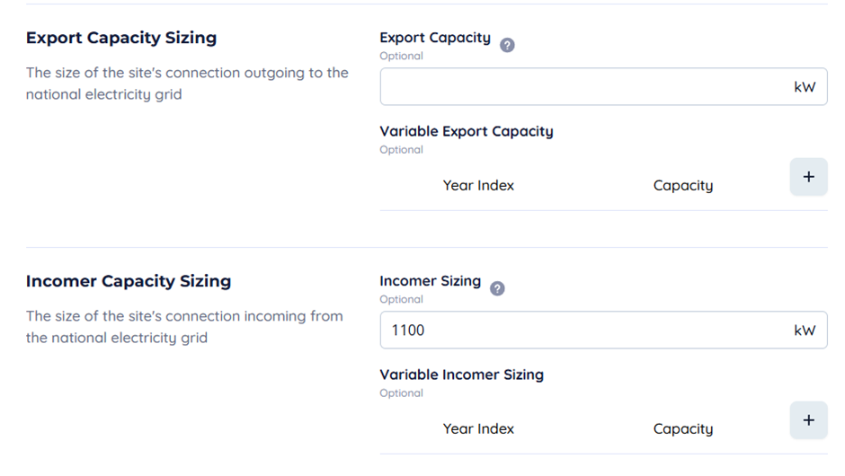
Both can vary over time; to represent upgrades to the site connection, you can add these by clicking the plus icon. Otherwise, the value will remain the same across the project if defined.

Headroom Analysis

Headroom analysis is accessible from the scenario page, below “Data” on the side navigation bar. To use it, select a year you want to analyse and hit “Refresh Data”; then the graph and table below it will repopulate.

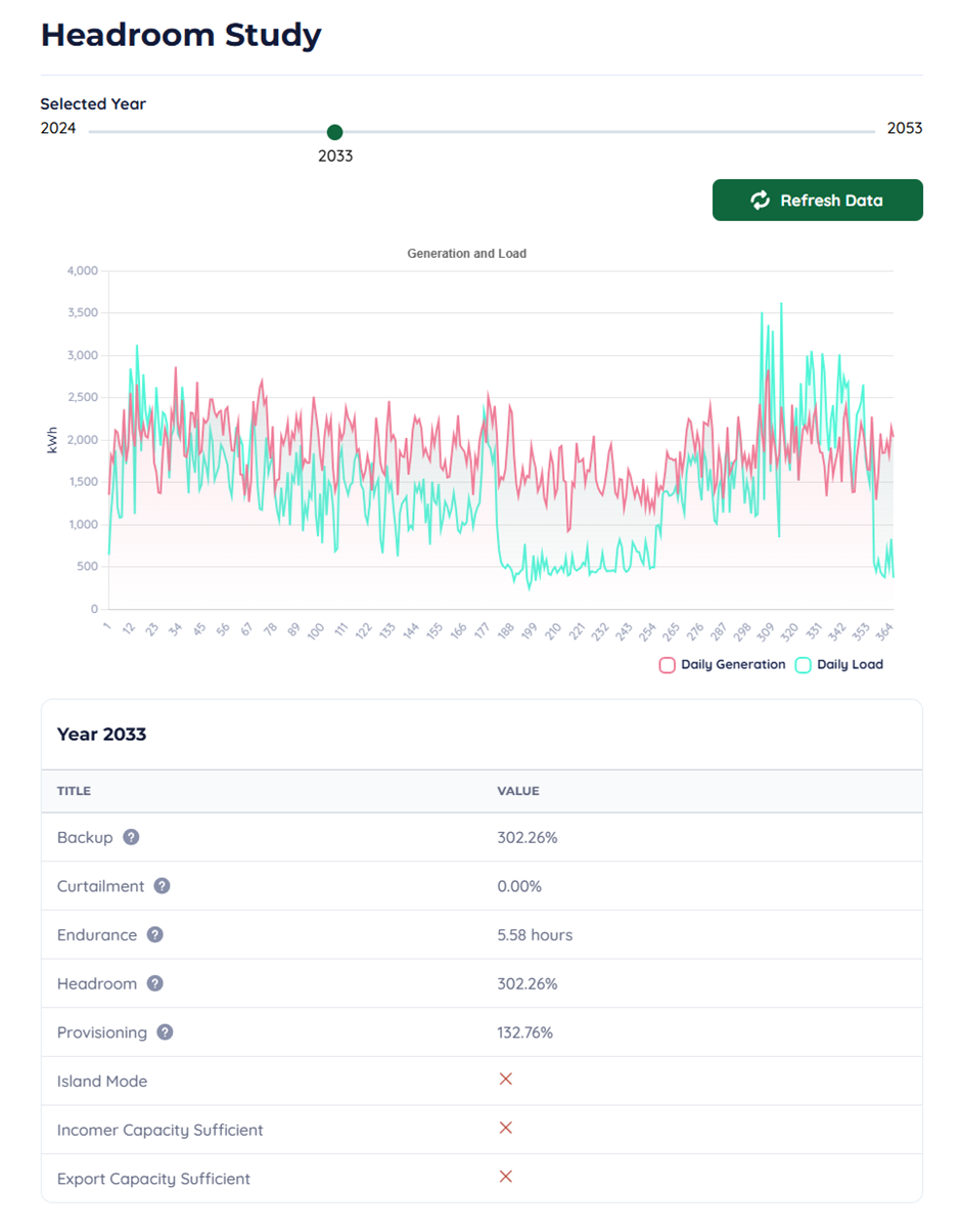
At first his might look overwhelming as there is a lot of information displayed on the screen. The three check marks at the bottom are the most critical. These determine whether your incomer or export sizing is enough. If the export sizing is not large enough, you will see curtailment; this can happen, for example, in large solar arrays. Likewise, if the incomer capacity is not enough, there is a point during the year when the amount of energy required to be imported exceeds the sizing of the incomer. By default, the frame length is a half-hour.

The “Island Mode” check represents the ability of the onsite generation to be able to meet all the electrical demands of the site. In other words, whether the amount of energy required to be imported never exceeds 0.

“Backup” is the percentage of the maximum demand that batteries and generators can supply if over 100% in the event of a power failure, the site is never projected to lose power. “Endurance” is the length of time the battery backups on site can last.

“Headroom” is the maximum generation added to the incomer size divided by the maximum demand. Now you may ask if this number greatly exceeds 100% why the island mode check isn’t true, this is because Encast models maintenance and a range of other dynamics across the model that can affect how individual installations behave. These times can be analysed in detail view.

“Provisioning” is whether the amount of energy generated annually could meet the demand. This only gives you an indication that it is enough, not that it does. If, for example, you have a high level of provisioning, but you do not satisfy the island mode check, you could add more batteries to the model. There are an innumerable number of factors and parameters you can use to adjust this which we will not get into detail with here.

Detail View

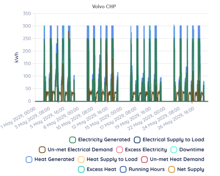
Detail view is the singularly most powerful analysis tool in Encast, it allows you to directly see up to four weeks of data. Select your scenario and your dates, then hit refresh to see into the model.

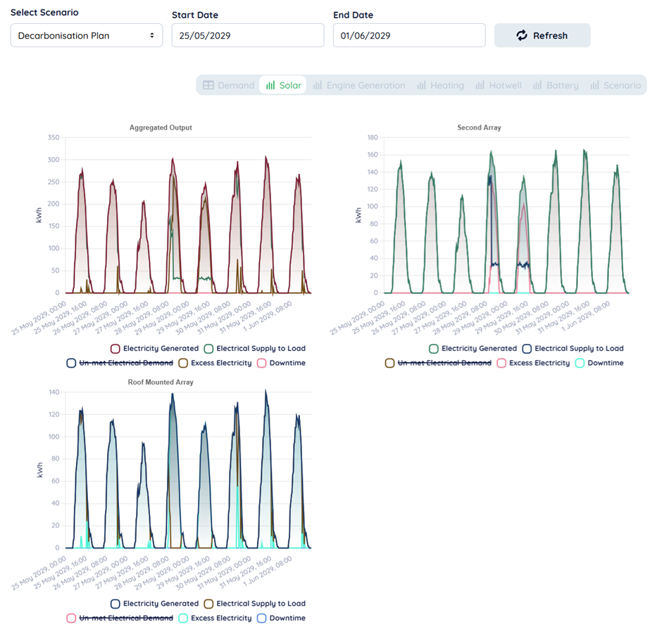
There are several tabs below the data selector one for each type of installation installed above is an example for the output of two arrays in a scenario. The aggregated output for each type of installation will be in the top left. You can click each series in the legend to turn the data off; this is useful to turn unmet demand off, which will often be much higher than the individual installations output.

As the data returned is used in the model itself, you can see all the effects of conditional operation events and maintenance all at once. The best way to do this for the entire project is to flip over the scenario tab.

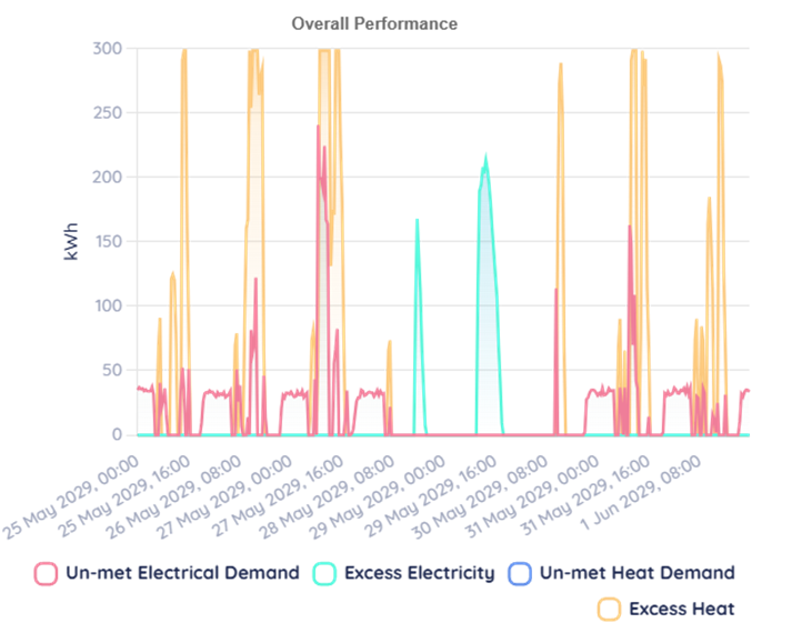
Here we can see that there is a shutdown on the 29th and 30th and there is excess electricity. So, we should see that any batteries in the project should charge on those dates, we can check this by going to the battery tab.

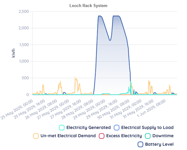
We can see the battery charges fully, indicated by the flat top on the graph. We could use this insight in any number of ways, and this should provide a demonstration of how to use this feature.

Heating

Heating is a separate network from electricity, as such it has its own associated modules and demands, however, as you might expect, CHP crosses over between them. Heat pumps and resistive heaters likewise use electricity to function.

Demand

To prevent confusion, heat demand value maps are segregated from electricity demands and profit and loss value maps.

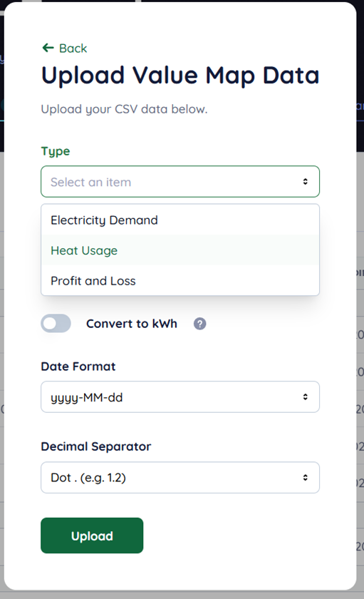
To upload a heat value map, change the type when uploading a csv; the same option appears for the other value map generators.

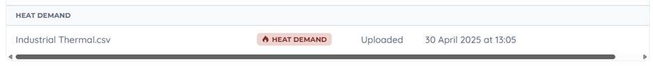
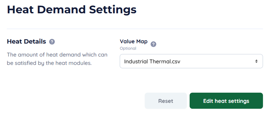
It should then appear with a different coloured label like so. Then you can navigate to heat demand and then either create a demand profile or alternatively use a value map that will run for the entire project.

CHP

Combined heat and power use the settings of an engine installation to generate heat when it runs, both liquid and gas engines can have CHP enabled though are calculated slightly differently.

Heat Storage – Hot Wells

Hotwells act similarly to batteries but have more parameters controlling their heat loss.

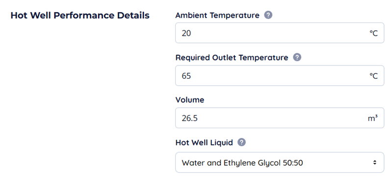
Ambient temperature is the average ambient temperature of the site. The required outlet temperature is the minimum required temperature of fluid exiting the hot well. Below this is will cease to function. The hot well liquid determines the maximum temperature the Howell can achieve in addition to the specific gravity of the liquid.

Because of how Encast is designed, all networks work on kWh, so the way in which temperature varies in the Hot Well may be unintuitive.

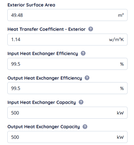
Exterior surface area and heat transfer coefficient determine how much heat is lost; this is a simple thermodynamic model. The heat exchanger efficiency and sizing operate similarly to batteries and limit the amount of input and output the hot well can take and how efficient the exchanger is.

Heat Sources

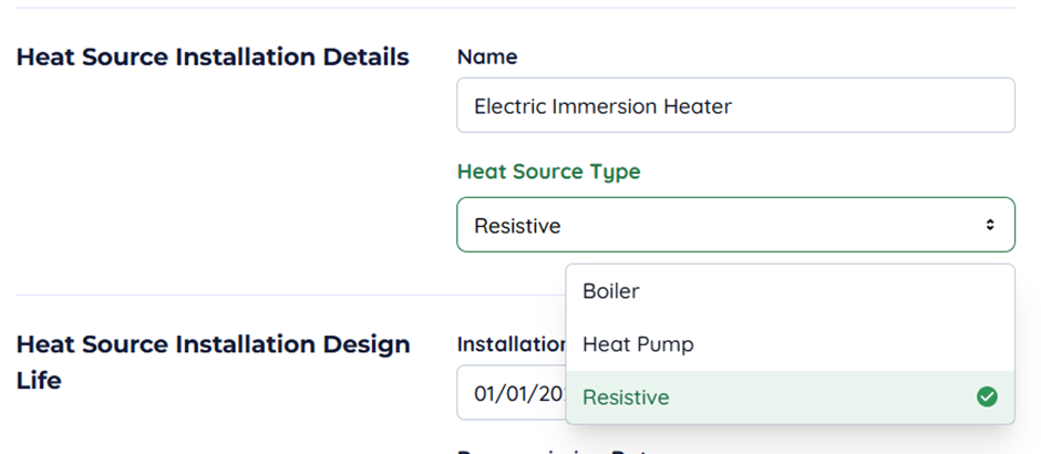
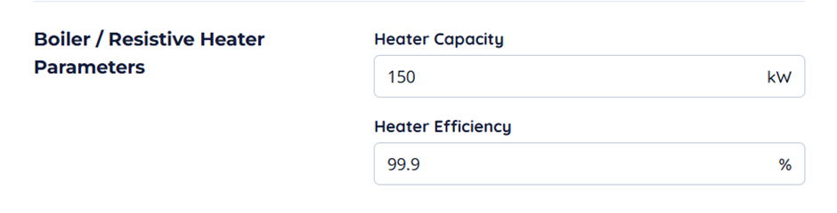
Heat sources are the collective term for the three different types of heaters available in Encast. These are resistive heaters, gas boilers, and heat pumps.

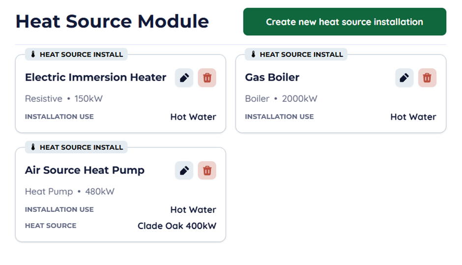
For resistive heaters and boilers, the capacity is just a simple capacity with an efficiency. Boilers have a variable that tracks gas use, resistive heaters contribute to the electrical load.

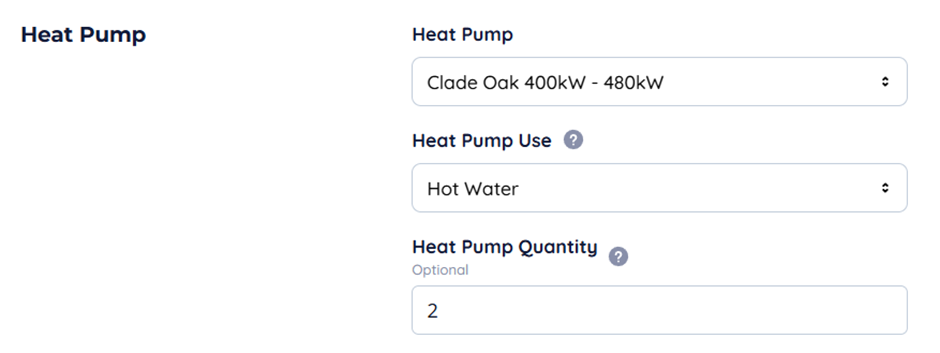
Heat pumps have a part associated with them which contain variables like seasonal coefficients of performance, hot water performance coefficient, and nominal capacity.

Binary operation means that the heat source is either on or off, this is useful for some types of resistive heaters controlled using only a relay. Off by default means that the heat source ignored normal demand and will only be triggered by operational criteria which are covered in a later tutorial.

Wind

Wind turbines work in a similar way to solar panel arrays; they ingest weather data to produce a reasonable estimate of wind performance at the given coordinates. There is a parameter called shade factor which acts as a scalar adjustment to wind speed at the hub height of the turbine.

The turbine model determines the performance; hub height is essential in some locations as the model incorporates wind speed at both the 10 m and 100 m level.

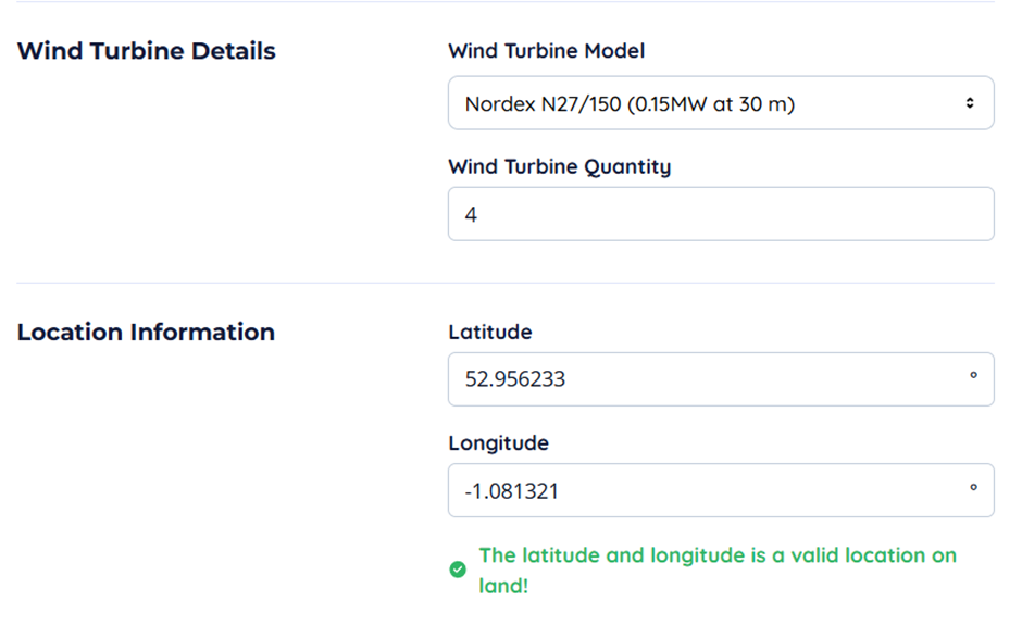
You can set the turbine quantity to whatever you wish, but it should be noted that Encast does NOT model interactions between turbines or terrain, so performance should be treated as a first order estimation.

Anaerobic Digestion / Biomass

Anaerobic digestion plants require a good deal of setup, however, can be a powerful tool in estimating yields ahead of time. It is a proprietary implementation of the US EPA’s “Anaerobic Digestion Screening Tool”.

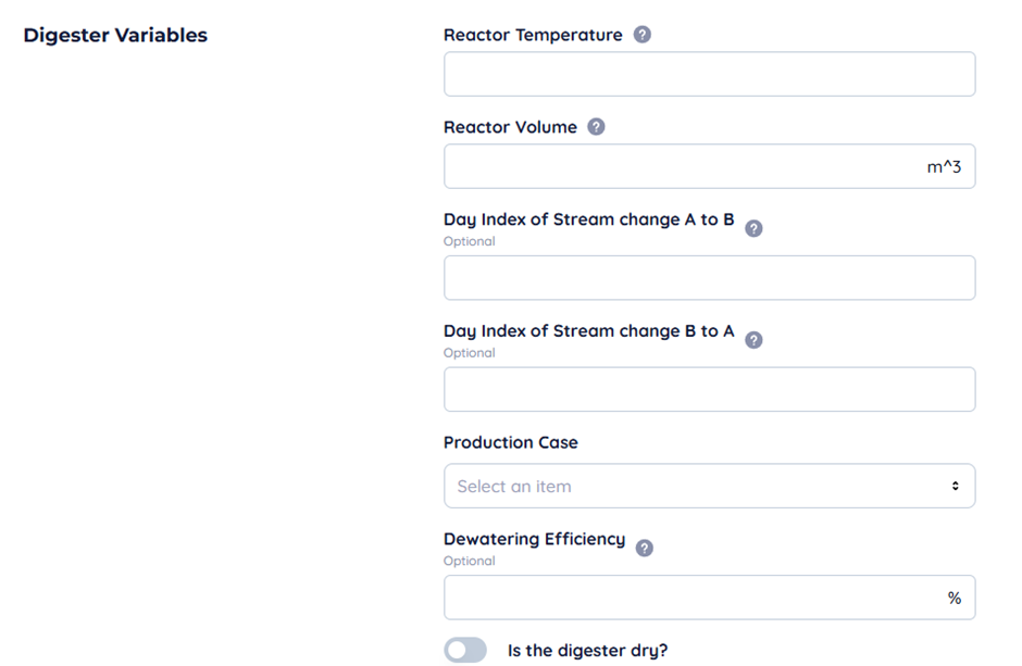
Reactor temperature will determine which regime of digestion the plant operates in.

• Unheated – between 10–20C
• Mesophilic – 30–40C
• Thermophilic – 50–60C

The temperature may affect the output in some gas production cases. Which are the low (25%) and high (75%) percentile values of the ratio between measured and modelled data. The maximum represents the theoretical maximum amount of gas the plant could produce.

Dewatering efficiency is the post-digestion efficiency of dewatering equipment, which will affect how much digestate the plant produces. If the digester is expected to contain between 15 and 40% dry solids, then you should check the relevant flag.

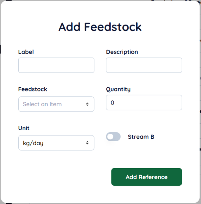
The correct mix of feedstocks is highly variable and an extremely complex topic, dealing with carbon/nitrogen ratios and toxicity. For not we will just go through entering a feedstock. Hit "add feedstock" and give it a label and description, select the feedstock and add a quantity. The unit will determine what the quantity is, so if you want 10 metric tons per day, type 10 in the quantity and change the unit.

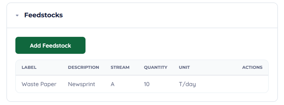
Once added, it will appear in the table. You can edit, copy, or delete each entry under actions. An important note you will need to hit save digester before these changes are saved. Do not navigate backwards or your work will be lost.

Maintenance

Maintenance allows you to periodically add both costs and a shutdown time as part of an installation’s operation. This can be done in the maintenance section in all installations create and edit pages.

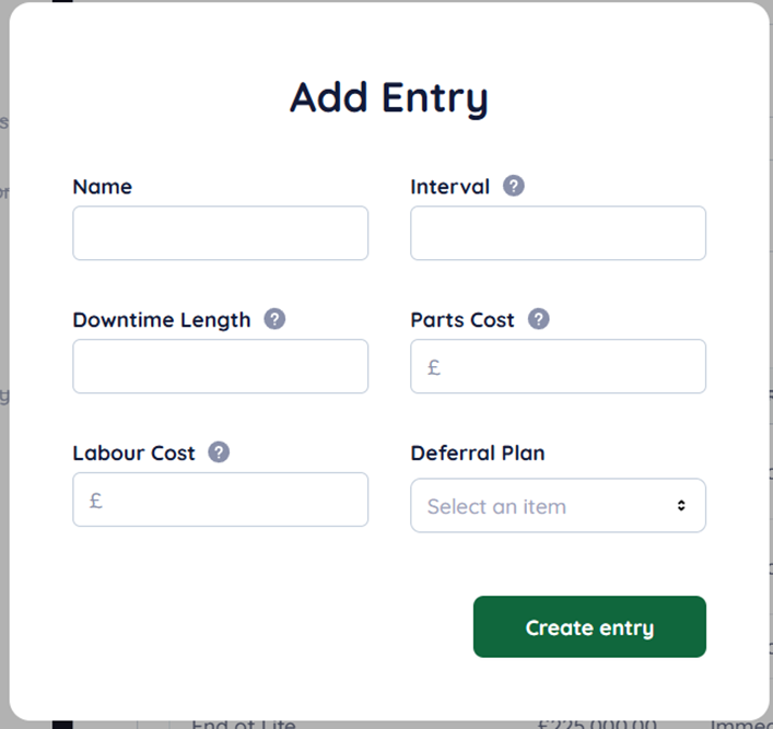
Add a name, an interval in running hours and a downtime length in hours. Parts and labour costs are used to populate the associated profit and loss entry.

A deferral plan must be selected, this is immediate, IE exactly when the running hours hit the interval, or deferred day which selects a day in the next week for the downtime to happen.

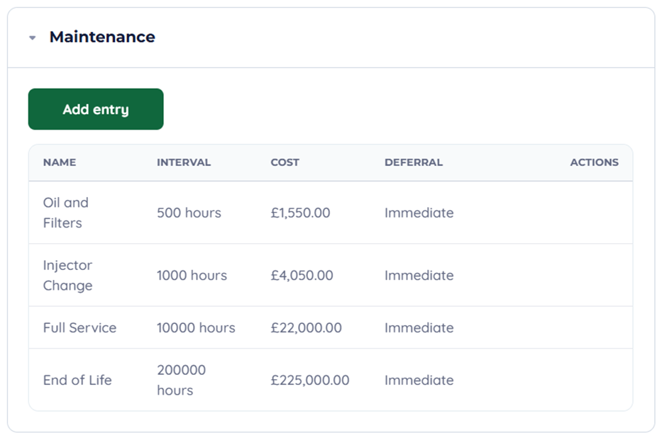
You can add as many as you wish, and you can edit clone or delete entries using the actions on the left side of the table.

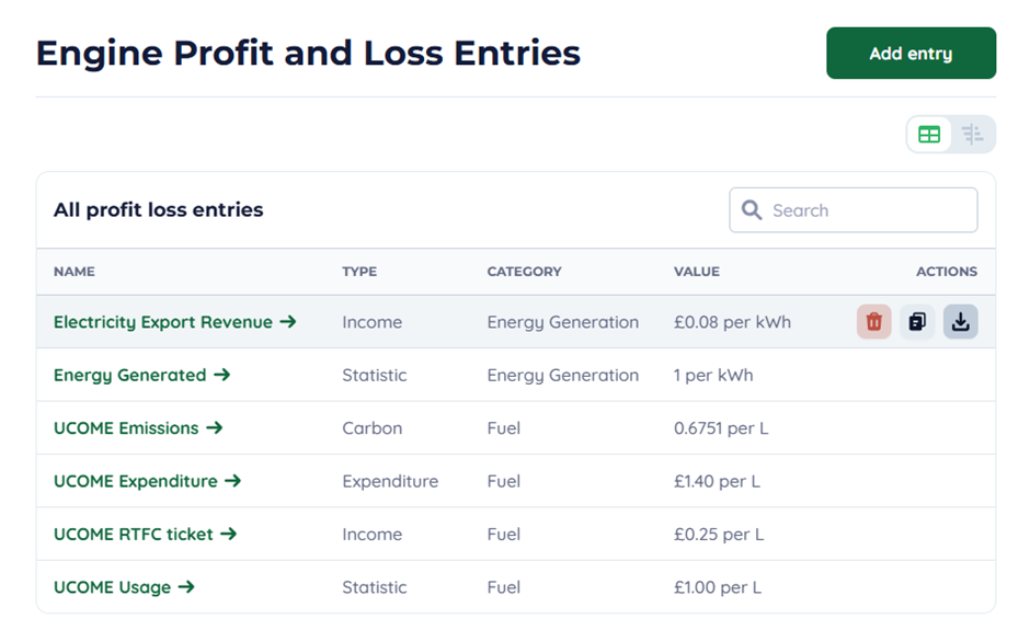
Excel Downloads

On every module page you can select the download action on each profit and loss entry.

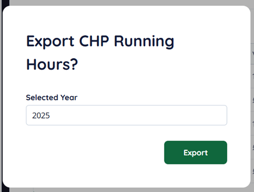
Then select the year you want to export.

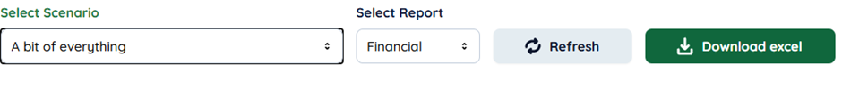
You can also export the financial report by pressing the button in the report tab.

Levelised Cost of Energy – LCOE

Levelised cost is a sophisticated tool to calculate the cost for each kWh of useful energy generated.

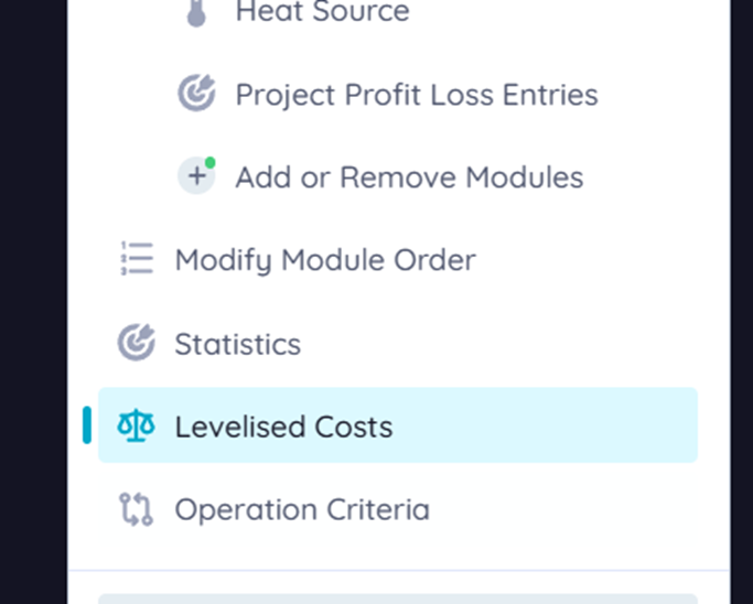
You can find levelised costs on the navigational sidebar, if you don’t have any, click “Create new levelised cost”

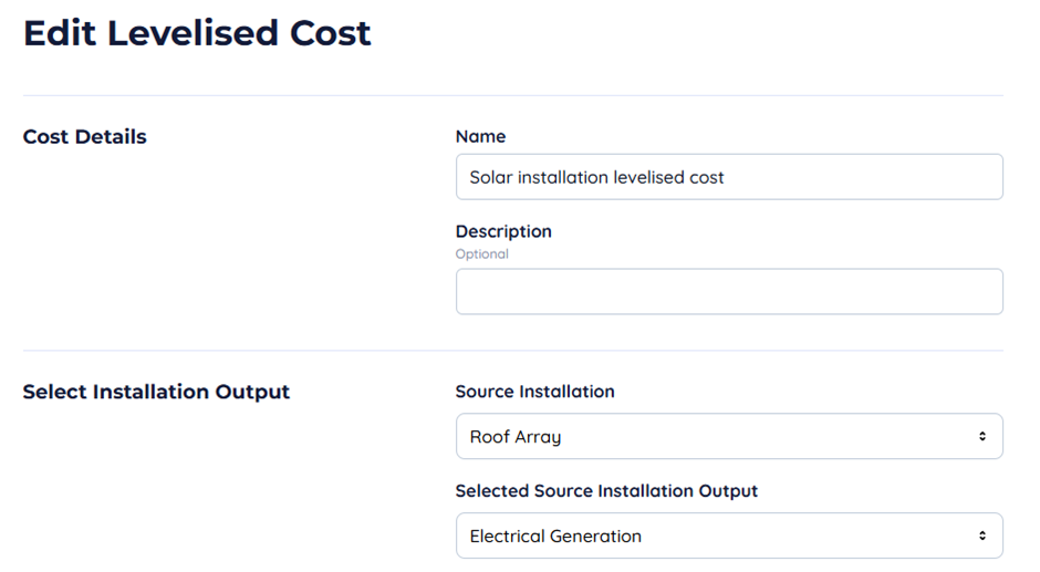
You will need to select which installation you want to analyse and which output you wish to calculate the cost against.

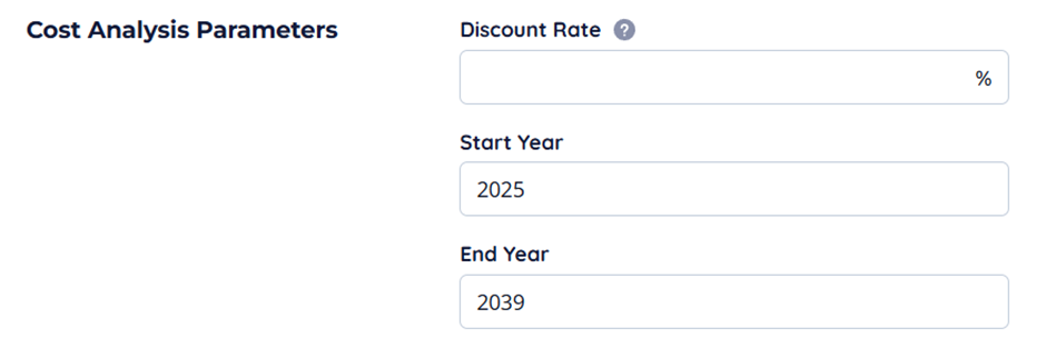
Select which years you wish to analyse and the discount rate across the analysis span. The discount rate presents the levelised cost as a net present cost of energy. By default, the start and end years of the project are selected.

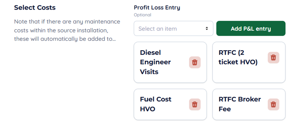
Any maintenance entries are automatically added; however, you can add the relevant fuel cost entries and other costs to the calculation. Here the RTFC is not a cost but a government subsidy which is taken of the cost.

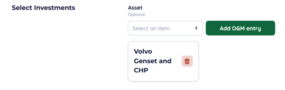
You can also add asset costs which again contribute to the cost of energy.

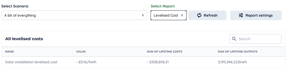
To access the outputs, go to the Reports tab and select the Levelised cost report. These costs are quite challenging to calculate, and you should be happy with your methodology on paper before attempting to model it in Encast.